Visualizing and Understanding Convolutional Neural Network

Visualizing and Understanding Convolutional Neural Network

どのように畳み込み層で処理がなされているか、という話。以前の疑問が少し和らいだ気がするけどまだストンと腹に落ちない、、、、

これらを使ってStyle Transferなど面白い応用につながる。

Several approaches for understanding and visualizing Convolutional Networks have been developed in the literature, partly as a response the common criticism that the learned features in a Neural Network are not interpretable. In this section we briefly survey some of these approaches and related work.

Neural netで学習を終えた重み・特徴量というものが理解に難しいという指摘がなされてきた、それに対する答えとして様々なアプローチが取られてきたようだ。

一つ目が重みをかけられた画像というものがどういうもの可視化するアプローチ

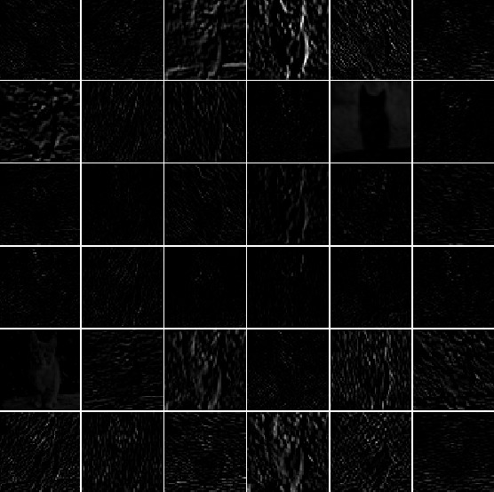
Layer Activations. The most straight-forward visualization technique is to show the activations of the network during the forward pass. For ReLU networks, the activations usually start out looking relatively blobby and dense, but as the training progresses the activations usually become more sparse and localized. One dangerous pitfall that can be easily noticed with this visualization is that some activation maps may be all zero for many different inputs, which can indicate dead filters, and can be a symptom of high learning rates.

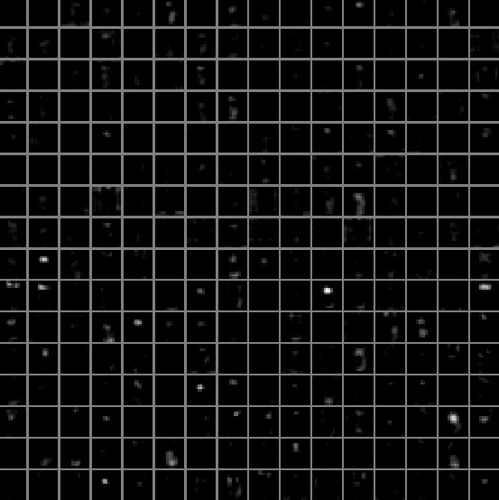Typical-looking activations on the first CONV layer (left), and the 5th CONV layer (right) of a trained AlexNet looking at a picture of a cat. Every box shows an activation map corresponding to some filter. Notice that the activations are sparse (most values are zero, in this visualization shown in black) and mostly local.

 

 

二つ目が重みを可視化するアプローチ

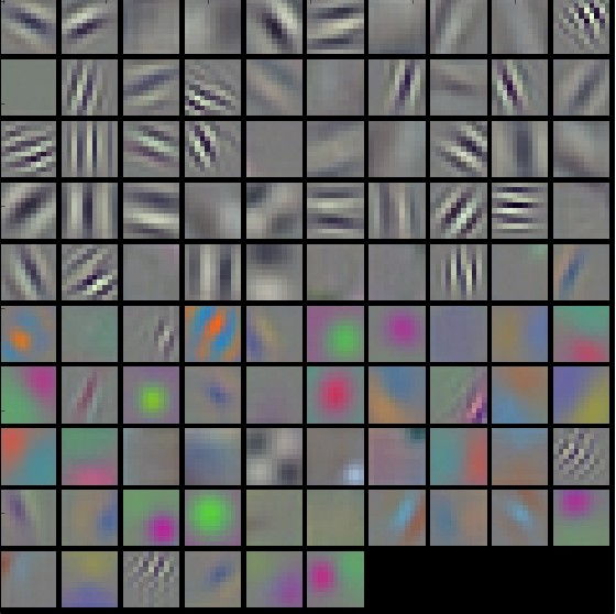
Conv/FC Filters. The second common strategy is to visualize the weights. These are usually most interpretable on the first CONV layer which is looking directly at the raw pixel data, but it is possible to also show the filter weights deeper in the network. The weights are useful to visualize because well-trained networks usually display nice and smooth filters without any noisy patterns. Noisy patterns can be an indicator of a network that hasn’t been trained for long enough, or possibly a very low regularization strength that may have led to overfitting.

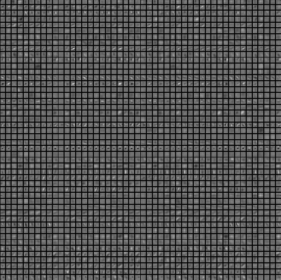Typical-looking filters on the first CONV layer (left), and the 2nd CONV layer (right) of a trained AlexNet. Notice that the first-layer weights are very nice and smooth, indicating nicely converged network. The color/grayscale features are clustered because the AlexNet contains two separate streams of processing, and an apparent consequence of this architecture is that one stream develops high-frequency grayscale features and the other low-frequency color features. The 2nd CONV layer weights are not as interpretable, but it is apparent that they are still smooth, well-formed, and absent of noisy patterns

Retrieving images that maximally activate a neuron

Another visualization technique is to take a large dataset of images, feed them through the network and keep track of which images maximally activate some neuron. We can then visualize the images to get an understanding of what the neuron is looking for in its receptive field. One such visualization (among others) is shown in Rich feature hierarchies for accurate object detection and semantic segmentation by Ross Girshick et al.:

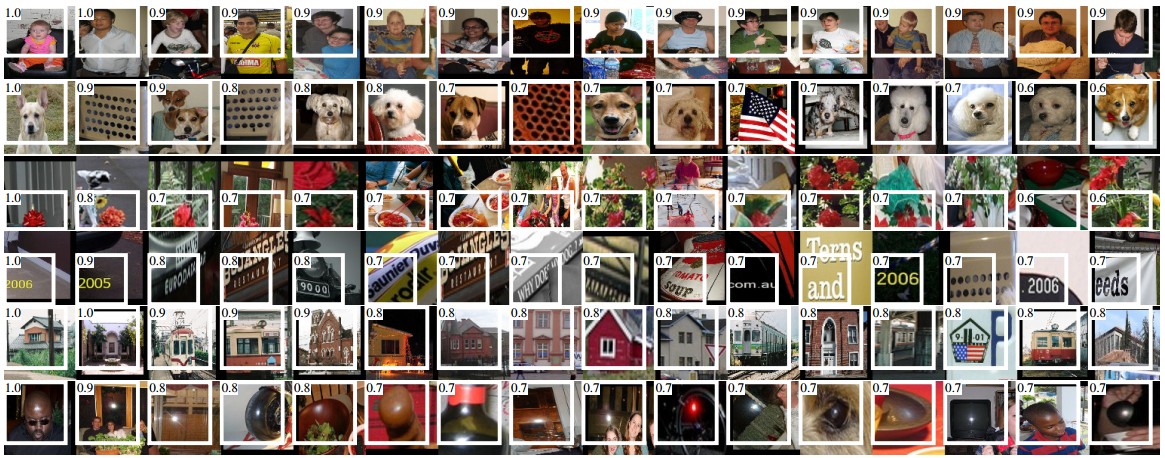Maximally activating images for some POOL5 (5th pool layer) neurons of an AlexNet. The activation values and the receptive field of the particular neuron are shown in white. (In particular, note that the POOL5 neurons are a function of a relatively large portion of the input image!) It can be seen that some neurons are responsive to upper bodies, text, or specular highlights.

One problem with this approach is that ReLU neurons do not necessarily have any semantic meaning by themselves. Rather, it is more appropriate to think of multiple ReLU neurons as the basis vectors of some space that represents in image patches. In other words, the visualization is showing the patches at the edge of the cloud of representations, along the (arbitrary) axes that correspond to the filter weights. This can also be seen by the fact that neurons in a ConvNet operate linearly over the input space, so any arbitrary rotation of that space is a no-op. This point was further argued in Intriguing properties of neural networks by Szegedy et al., where they perform a similar visualization along arbitrary directions in the representation space. 

 どのように画像が分類されるかを次元削減したのがt-SNEという手法

隣り合う画像は似たようなものとしてCNNに認識されているようだ。

Embedding the codes with t-SNE

ConvNets can be interpreted as gradually transforming the images into a representation in which the classes are separable by a linear classifier. We can get a rough idea about the topology of this space by embedding images into two dimensions so that their low-dimensional representation has approximately equal distances than their high-dimensional representation. There are many embedding methods that have been developed with the intuition of embedding high-dimensional vectors in a low-dimensional space while preserving the pairwise distances of the points. Among these, t-SNE is one of the best-known methods that consistently produces visually-pleasing results.

To produce an embedding, we can take a set of images and use the ConvNet to extract the CNN codes (e.g. in AlexNet the 4096-dimensional vector right before the classifier, and crucially, including the ReLU non-linearity). We can then plug these into t-SNE and get 2-dimensional vector for each image. The corresponding images can them be visualized in a grid:

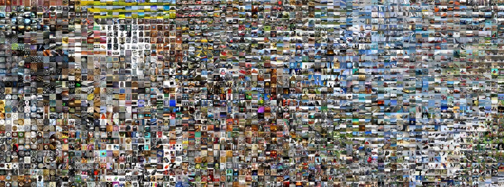t-SNE embedding of a set of images based on their CNN codes. Images that are nearby each other are also close in the CNN representation space, which implies that the CNN "sees" them as being very similar. Notice that the similarities are more often class-based and semantic rather than pixel and color-based. For more details on how this visualization was produced the associated code, and more related visualizations at different scales refer to t-SNE visualization of CNN codes.

一部の画像を穴あき状態にして、正しく分類される確率はどうかと可視化することで、その画像のどこが重要となっているかを示すのが次の手法

Occluding parts of the image

Suppose that a ConvNet classifies an image as a dog. How can we be certain that it’s actually picking up on the dog in the image as opposed to some contextual cues from the background or some other miscellaneous object? One way of investigating which part of the image some classification prediction is coming from is by plotting the probability of the class of interest (e.g. dog class) as a function of the position of an occluder object. That is, we iterate over regions of the image, set a patch of the image to be all zero, and look at the probability of the class. We can visualize the probability as a 2-dimensional heat map. This approach has been used in Matthew Zeiler’s Visualizing and Understanding Convolutional Networks:

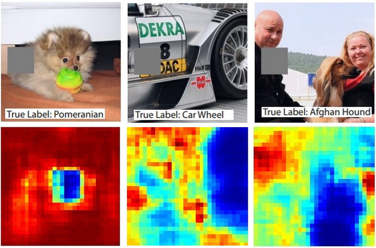Three input images (top). Notice that the occluder region is shown in grey. As we slide the occluder over the image we record the probability of the correct class and then visualize it as a heatmap (shown below each image). For instance, in the left-most image we see that the probability of Pomeranian plummets when the occluder covers the face of the dog, giving us some level of confidence that the dog's face is primarily responsible for the high classification score. Conversely, zeroing out other parts of the image is seen to have relatively negligible impact.

今回はコピペばっかりになってしまった

cs231n.github.io

Detection and Segmentation

Detection and Segmentation

これらは今までの画像分類の技術を駆使するという感じである。

分類して、それがどこにあるのかというところまで示す。

traindata にはカテゴリーと座標が与えられそれを学習する。

その上でどのように計算量を減らすかというような工夫がなされている。

これから研究されるテーマであるようだ。

近況報告 イスラエル行ける！！

CS231nの講義もlecture12まで見終わり、いよいよとりあえず１周ができそう。

ライブラリにも慣れたいのでpytorchのtutorialも写経しながらとりあえず触れてみるという感じ、まだよくわからない泣

プログラミング歴も浅くコードを解釈する力も足りず、、、泣

でもまあ頑張っていきます

先日大学の授業でデータ分析の結果発表会があり、幸運なことに優秀者に選ばれ教授とイスラエルに研修行けることになりました！！

それまでにはガッキーでディープラーニングして成果を出し、研修先で発表できたりするといいな〜などと妄想してます。

先日4000枚のガッキーの画像を集めました、ガッキー可愛い

考えている手順としては

CNNで分類する　ガッキーと堀北真希、堀未央奈、僕の自撮りを分類するのを作りたい
GANで画像生成　ガッキーを画像生成

GANで画像生成　ガッキーと堀北真希、堀未央奈を組み合わせた絶世の美女を生成したい

頑張るぞ〜

RNN Recurrent Neural Networkについて

RNN Recurrent Neural Networkについて

深層学習　(岡谷貴之著)によると、再帰型ニューラルネット（Recurrent Neural Network）とは 

再帰型ニューラルネット(RNN )は、音声や言語、動画像といった系列データを扱うニューラルネットです。これらのデータは、一般にその長さがサンプルごとにまちまちで、そして系列内の要素の並び(文脈)に意味があることが特徴です。RNNは、このような特徴をうまく取り扱うことができます。

また

再帰型ニューラルネット(RNN)は、内部に(有向)閉路を持つニューラルネットの総称です。RNNはこの構造のおかげで、情報を一時的に記憶し、また振る舞いを動的に変化させることができます。これにより、系列データ中に存在する「文脈」をとらえ、上述のような分類問題をうまく処理できるようになります。

Model Ensemble モデルアンサンブルについて

Model Ensemble モデルアンサンブルについて

実用上一通り学習を終えた後にもう一つ精度を上げたいとなった場合、モデルアンサンブルという手法がとられることがある

この手法は、最後の予測を複数のモデルの出力の平均をとった値を出力とする、という手法である。

Model Ensembles

In practice, one reliable approach to improving the performance of Neural Networks by a few percent is to train multiple independent models, and at test time average their predictions. As the number of models in the ensemble increases, the performance typically monotonically improves (though with diminishing returns). Moreover, the improvements are more dramatic with higher model variety in the ensemble. There are a few approaches to forming an ensemble:

• Same model, different initializations. Use cross-validation to determine the best hyperparameters, then train multiple models with the best set of hyperparameters but with different random initialization. The danger with this approach is that the variety is only due to initialization.
• Top models discovered during cross-validation. Use cross-validation to determine the best hyperparameters, then pick the top few (e.g. 10) models to form the ensemble. This improves the variety of the ensemble but has the danger of including suboptimal models. In practice, this can be easier to perform since it doesn’t require additional retraining of models after cross-validation
• Different checkpoints of a single model. If training is very expensive, some people have had limited success in taking different checkpoints of a single network over time (for example after every epoch) and using those to form an ensemble. Clearly, this suffers from some lack of variety, but can still work reasonably well in practice. The advantage of this approach is that is very cheap.
• Running average of parameters during training. Related to the last point, a cheap way of almost always getting an extra percent or two of performance is to maintain a second copy of the network’s weights in memory that maintains an exponentially decaying sum of previous weights during training. This way you’re averaging the state of the network over last several iterations. You will find that this “smoothed” version of the weights over last few steps almost always achieves better validation error. The rough intuition to have in mind is that the objective is bowl-shaped and your network is jumping around the mode, so the average has a higher chance of being somewhere nearer the mode.

同じモデルだが初期設定の値を変える方法

cross validationで良い精度の上からいくつかのモデルを使用する方法

学習にコストがかかってしまう場合、あるepoch数での状態のモデルを保存してそれらの平均を取る方法

がある。

ただしモデルアンサンブルはtestdataに対し出力するのに時間がかかってしまうらしい。

それを効率化する研究もなされているようだ。

One disadvantage of model ensembles is that they take longer to evaluate on test example. An interested reader may find the recent work from Geoff Hinton on “Dark Knowledge” inspiring, where the idea is to “distill” a good ensemble back to a single model by incorporating the ensemble log likelihoods into a modified objective.

cs231n.github.io

学習を上手く行うために Hyperparameter optimization ハイパーパラメーターの設定について

Hyperparameter optimization ハイパーパラメーターの設定について

Learning Rateやlearnig rate scheduleやregularization strengthなど調整すべきハイパーパラメーターをどのように設定するか

Learning Rateを例にとってまとめる

まずざっくりの範囲でRandom searchを行う

For example, a typical sampling of the learning rate would look as follows: learning_rate = 10 ** uniform(-6, 1).

このようにざっくり値を定めて

Prefer random search to grid search. As argued by Bergstra and Bengio in Random Search for Hyper-Parameter Optimization, “randomly chosen trials are more efficient for hyper-parameter optimization than trials on a grid”. As it turns out, this is also usually easier to implement.

良い精度を出す範囲を絞って行く

その絞って行く過程をどのようにするか

Stage your search from coarse to fine. In practice, it can be helpful to first search in coarse ranges (e.g. 10 ** [-6, 1]), and then depending on where the best results are turning up, narrow the range. Also, it can be helpful to perform the initial coarse search while only training for 1 epoch or even less, because many hyperparameter settings can lead the model to not learn at all, or immediately explode with infinite cost. The second stage could then perform a narrower search with 5 epochs, and the last stage could perform a detailed search in the final range for many more epochs (for example).

10の(−６~1)乗の範囲で探索している場合、多くても1epochで絞り込む

次の絞り込みの段階では5epoch

次の段階ではより多くのepoch数で範囲を絞って行く

cs231n.github.io

CNN Architectures VGGNet,AlexNet,GoogleNet,ResNetのケーススタディ

今回はCNNの様々なモデルについて書きとめようと思う。

VGGNetはそれまで首位を獲得していたAlexNetと比べ

より層を深くし、重みフィルターのサイズも小さくしている
Layer数 AlexNet 8 →VGGNet 16~19

重みフィルター（Conv層)

3×3, stride1,zero-padding1

Pooling

2×2,stride2

以前にも書き留めたが、重みフィルターを小さくすることには様々な利点がある。

7×7のConv層を1層重ねるのと、3×3のConv層を3層重ねるのは、見ている範囲（ピクセル数）は同じである。

しかし3×3のConv層を3層重ねると

非線形性をより表現でき、調整するパラメーター数を少なくすることができる。

GoogleNet
22Layer,

Inception Moduleという計算を効率よく行う工夫がなされている。

Inception Moduleでなされている工夫は、

Inputに対し複数の畳み込みを行い、次の層へと渡すということがなされる

しかし保持するParameterがとても大きくなってしまうため、

このように1×1の畳み込み層を挟んでから次の畳み込み層へ渡している。

この1×1の畳み込み層をbottleneck Layerと呼ぶ。

Fully ConnectedLayerは取り除かれている

さらに分類を行う処理を三つ取り入れている。

AlexNetに比べて約12分の1のparameter数である。

これらの工夫はBatch Normalizationが発明されていないためになされたものだが、BatchNormalizationを使えばこのような構造を取る必要はなくなるようだ。 

ResNet

152層も重ねている 

しかし普通層を重ねすぎると弊害が起こる

それは過学習を起こしてtestdataに対して低いスコアを出すということではなかった。

Optimization、重みの最適化の段階でうまく機能していないという問題点があった

解決策として

 residualと呼ばれる考えを使用しているらしい（理解に時間がかかる、、、）

他にもこれらを組み合わせた構造があるようだ。